Summary
Key questions
- What methods are available for evaluating energy efficiency policies in the transport sector?
- What are some best practice examples of evaluations of EU energy efficiency policies in the transport sector?
- What factors should be considered when selecting the most appropriate evaluation methodology?
Lead authors: Samantha Morgan-Price (Ricardo)
Reviewers: Bruno Lapillonne (Enerdata), Didier Bosseboeuf (Ademe)
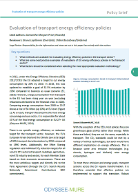
In 2012, under the Energy Efficiency Directive (EED) 2012/27/EU the EU adopted a target to cut energy consumption by 20% by 2020. In 2018, this was updated to establish a goal of 32.5% reduction by 2030 compared to business as usual scenario (EC, 2018). However, energy consumption from transport in the EU has been rising year on year (excluding reductions attributed to the financial crisis in 2008). Comparing energy consumption from 2000 to 2017 shows a rise of 34 Mtoe (up 10%) at EU level (Figure 1). As a result, transport has become the most energy consuming end-use sector; it is responsible for about 33 % of the final energy consumption in EU-27+ UK (Odyssee-MURE, 2020).
There is no specific energy efficiency or reduction target for the transport sector, however, the EU’s European Green Deal and the Climate Law set a target of 90% transport decarbonisation by 2050 compared to 1990 levels. Additionally, the Effort Sharing regulation sets individual CO2 reduction targets for all non-EU ETS sectors (transport, buildings, agriculture, non-ETS industry and waste), for each Member State based on their economic circumstances. These are the most ambitious targets and directly link to the Paris Agreement (through the EU’s Search Results Nationally Determined Contributions NDC commitment).
Figure 1 Energy consumption trends in transport (international aviation included) in EU27 +UK
 in EU27 +UK")
Source (Odyssee-MURE, 2018)
With the exception of the EED, most policies focus on greenhouse gases (GHG) rather than energy. While these are linked, they are not the same, especially in transport. The CO2 standards could be met by a variety of vehicle technologies, but each would have different implications on energy efficiency. This is because some zero emission technologies (e.g. electric, hydrogen and biofuels) raise energy consumption.
To meet these emission and energy goals, transport systems across the EU require transformation. It is therefore essential that effective policies are implemented to support this transition. Robust evaluations are crucial to understand how effective existing policies have been and to facilitate improvements in effectiveness for transport policies in the future.
According to the MURE database, only 130 of 547 (24%) transport measures in the EU have been evaluated in some way, and only 107 (82%) of these included quantitative estimates of GHG emission impacts (2018). This policy brief therefore provides an introduction on options and methods for evaluating the effectiveness of transport policies.
Sources of energy consumption
There are a number of aspects to consider when reviewing transport energy consumption. Traditionally, the use phase (e.g. when a vehicle is being driven) has accounted for the most significant proportion of a vehicle’s energy consumption and GHG emissions. However, as the automotive industry has moved towards alternative fuels, other phases are becoming more important. These include the production of vehicle and fuels and disposal phases. An electric vehicle’s impacts, for instance, will depend on the energy (and carbon) intensity of the electricity supply used to run the vehicle and used in the electricity intensive battery manufacturing process.
Types of energy efficiency measures in transport
The A-S-I Approach describes the three key policy types which seek to improve energy efficiency in the transport sector (ELTIS, 2014):
- Avoid – policies that reduce travel or the need for travel. Mainly achieved through land use planning, urban design or changing working arrangements (e.g. remote/tele-working).
- Shift – policies to increase shares of trips made on more efficient modes. This includes promoting cycling, walking and public transport as well as discouraging single occupancy vehicle use. Therefore, this policy type is often described in terms of energy per passenger km or tonne km.
- Improve – Includes technological improvements to increase vehicle and fuel efficiency, this includes adopting more efficient fuels. Economic/taxation measures can also encourage improvement, by prioritising less powerful options.
According to the MURE database, the majority of transport policies aim to support modal shift to public transport or improve inter-urban and urban traffic management. Regarding improve policies, over half of the measures in MURE aim to promote cleaner fuels (MURE 2020). These trends are understandable, as several policies may be needed to encourage successful shift from multiple other modes, whereas technological improvements can be controlled by setting just a few binding industry standards. Avoid policies tend to fall within the jurisdiction of urban planning, IT or employment policies. Therefore, shift and improve are most relevant to consider in transport policy.
Evaluation Approaches
A wide range of evaluation methods can be used to estimate the GHG effects of policies and actions. They can broadly be grouped into two categories:
- Bottom-up methods calculate the change in energy or GHG emissions for each source (e.g. vehicle) affected by the policy or action and then aggregate these across all sources (e.g. all vehicles in fleet) to determine the total change. Bottom-up data is typically measured, monitored, or collected (for example, using a measuring device such as a fuel meter) at the energy consumption source level.
- Top-down methods consider the amount of energy saved at a larger, aggregated scale (e.g. national, or sectoral). These approaches begin with global level data (e.g. national statistics for energy consumption or use of a specific technology) and disaggregate ‘down’, to assess the savings coming from different factors (e.g. energy price, autonomous progress, market forces). These methods can be used to reveal trends in data and, depending on the level of disaggregation possible, can sometimes attribute energy savings to policies or package. For example, the impact of policies promoting low-carbon fuels and technologies can be understood from data on the sales of the low-carbon fuel data. However, if multiple polices are aiming to target the same low-carbon fuel/technology, top down methods cannot split the impacts between policies
Bottom up and top down methods are complementary. Top down provide total savings and bottom up provide the policy’s attributed savings. The nature of transport policy, especially for cars, highlights the importance of both approaches. As many policies focus on cars, thus evaluations tend to focus on packages of measures. Technical driven savings are easier to evaluate (e.g. using stock modelling) whereas modal shift policies are more complex for bottom up methods
Table 1 presents MURE’s categorisation of evaluation methods into bottom-up, top-down or a combination of the two. It also shows their frequency of use across the 30 countries who contribute to the MURE database. Hybrid methods appear to be the most common, with 78 evaluations utilising these types of methods. Econometric modelling (top-down) is less common with only 6 studies reported in the MURE database.
Table 1 Evaluations methods and number of evaluations that feature them in the MURE database (contains submission from EU27 countries + Norway, Switzerland and UK) (source: http://www.measures-odyssee-mure.eu/)
| Methods | Description | # studies | |
|---|---|---|---|
| Bottom-up | Direct measurement | Monitoring of types of fuels used by a particular source, to understand changes in usage caused by a policy. | 14 |
| Billing analysis | Analysis of energy or fuel bills of a particular source can show changes in energy use. | 0 | |
| Enhanced engineering estimates | Estimate energy savings collected ‘at source’ of energy consumption and distance travelled by source, either using specialised testing equipment or by monitoring end-use actions. | 17 | |
| Mixed deemed ex-post estimate | Energy estimates understood by tracking equipment sales data, inspecting samples and monitoring equipment purchased and combining with real world use. For example, official fuel consumption and CO2 emissions data of all new road vehicles are measured before they can be sold. | 73 | |
| Deemed estimate unit savings | Detailed engineering estimates conducted via a model or simulation. This involves a similar approach to the mixed deemed estimate, but the analysis will also consider samples taken before the implementation of the measure being implemented. For example, used to evaluate white certificates (EC, 2020). | 18 | |
| Bottom-up and/or Top-down | Stock modelling | Considers vehicle stock (supply) and user patterns to understand the impact of policies. It can be either bottom-up or top-down. It is particularly useful in transport but can be complex to apply. Typically, a bottom-up model would be able to simulate activity and traffic flows resulting from drivers of activity (e.g. user demand, transport infrastructure) and combine with fuel use and sources. Without user demand patterns, it becomes a top-down approach. | 18 |
| Diffusion indicators | Diffusion indicators describe the share of equipment (vehicles) or practices within a market. It can be bottom-up by using an indicator of uptake in a market that is only changed by the specific measure (e.g. few examples from transport, however installation of smart meters in households is a suitable uptake indicator for buildings sector). Otherwise, it will be top-down (e.g. EV promotion where it is common to have multiple policies supporting uptake). | 0 | |
| Top-down | Consumption indicators | Analysis centred on monitoring of energy consumption indicators (e.g. volume fuel used in freight transport) for whole sector, sub sectors or transport modes. | 14 |
| Econometric modelling | Combines economic data and statistical modelling to understand the relationship between variables. Examples include regression analysis (see case study below for more information) and Input/Output (I/O) analysis (macroeconomic analysis based on the interdependencies between economic sectors or industries). | 6 | |
| Hybrid | Integrated bottom-up & top-down | Also known as hybrid models, these combine top-down and bottom-up methods to disaggregate data and analysis further than in typical top-down methods, but does not achieve the same level of detail as bottom-up methods. | 78 |
Case Studies
The following section presents two best practice applications of evaluation methods well-suited to reviewing energy impacts and trends in transport. The first is an econometric (regression) analysis, which, according to MURE, is used infrequently. The second example is a decomposition analysis, which is a top-down method which can be used to study trends in energy demand of a sector or sub sector.
Regression analysis can attribute impacts and changes to specific causes, including policies. Decomposition analysis disaggregates changes in energy use into pre-defined sector specific drivers.
Method 1: Econometric (regression) analysis
Box 1 below contains a case study of econometric analysis applied in an evaluation of an EU-level transport policy.
Box 1 Case study 1: Evaluation of Regulations 443/2009 and 510/2011 on CO2 emissions from light-duty vehicles (DG CLIMA, 2015)
This evaluation considered two separate regulations that aim to reduce GHG emissions from road transport by setting mandatory fleet-based CO2 reduction targets (in gCO2/km) to new cars (Regulation (EC) No 443/2009) and Light Duty Vehicles (LDVs) (Regulation (EU) No 510/2011). The evaluation sought to understand the effectiveness, cost and resource efficiencies.
Method: The impact of the regulations was assessed using an econometric approach. This involves understanding variables connected to the impacts and identifying those which are dependent on the regulation. The analysis then aims to quantify how a dependent-variable changes when one of the independent variables (i.e. explanatory variable) is varied while the other independent variables are held fixed. Therefore, the analysis removes the impacts of other factors that may have had an impact on emissions from new vehicles, so that only remaining change in CO2 emissions can be attributed to the regulations.
Factors effecting CO2 reductions related to the policy, were categorised as: a) Time dependent variables; b) Outcome variables that can impact on the outcome of analysis (e.g. CO2 emissions of new cars/LDVs) but are not a direct consequence of the regulations. c) Omitted variables that correlate with the policy but are not casually linked (e.g. consumers’ preferences). d) Anticipation variable reaction to policy by key actors1. The final change observed in emission and energy usage was adjusted by removing these variables. The remaining change observed can then attributed to the policies.
Results: The results suggest that around two-thirds of the reductions observed since 2009 can be attributed to the Regulation. Specifically, 65% of improvements in energy efficiency was attributed to the Regulation (equivalent to 3.5 gCO2/km). Whereas, autonomous improvement led to a 33% (~1.6 gCO2/km) reduction. These results indicate analysis indicates that the regulation has been more successful in reducing emissions than the voluntary agreement that was previously in place.
Method 2: Decomposition analysis
Decomposition analysis methods ‘decompose’ a target variable into pre-defined factors and then determines their contribution to the overall target value. These drivers do not necessarily directly relate to individual policies; the impacts of a specific policy are only indirectly visible through the changes in the drivers (see Box 2 below).
Box 2 Case study 2 : Understanding variation in energy consumption using decompossion analysis (ODYSSEE-MURE, 2020) (EC, 2020)
Decomposition analysis is conducted as part of the ODDYSSEE-MURE project, and available via an online tool. The objective of this tool is to explain the variation of the energy consumption over a given period through a decomposition into certain factors. This case study will focus on the transport results only.
Method: The pre-defined drivers of energy consumption in decomposition method are activity (i.e. km-passenger or km-tonne, modal shift (i.e. the structure of transport split by mode), efficiency (or energy savings consumption per passenger or tonne kilometre by mode) and ‘other’ effects.
Results: Energy use since 2000 in transport was found to have increased by 34 Mtoe. This change in energy consumption is attributed to the identified key drivers in Erreur ! Source du renvoi introuvable.2. Activity increases in passenger (including international aviation) and freight transport contributed an additional 79 Mtoe. This effect was counterbalanced by energy savings (i.e. improvements to the efficiency of vehilces) which contributed to decrease the energy consumption by 57 Mtoe. Other effects (e.g. ‘negative savings’ in freight transport due to low capacity utilization) increased the energy consumption by 7.9 Mtoe. Modal shift had a minor increasing effect of about 4.3 Mtoe, 4.1 Mtoe of which occurred in freight transport. This impact is likely to be smaller than what would have occurred without policies avoiding shift to less efficient modes, indicating some level of success from these policies. Additional (bottom-up) analysis would be required to attribute this to individual policies.
Figure 2 changes in final energy consumption of transport between 2000 and 2017.

The table below compares the characteristics and applicability of the two methods.
Table 2 Method applicability comparison
| Regression analysis | Decomposition analysis | |
|---|---|---|
| Type of method | Analytical, quantitative and flexible. | Analytical and quantitative. Predefined structure of analysis and results. |
| Evaluation focus | Understanding impacts of a particular policy or package. | Sector, sub sector or mode. Not suitable for understanding impacts of a policy or package. Effectiveness only indirectly attributable to PaMs. |
| Policy types | Wide applicability, but particularly suited to fiscal incentives (e.g. tax exemptions). | Suitable for providing overall of trends for demand and supply transport policy. Applicable at mode or fuel type level. It is not possible to remove external factors without combining with other methods. |
| Level | Both can be applied to regional, country or city/municipality levels, dependent on data availability. | |
| Sector disaggregation | Applicable to any disaggregation, depending on data availability. | Mode, activity types, fuel type and efficiency of vehicles. |
| Data requirements | Mainly suitable when detailed, high quality data is available. Public data would need supplementing with policy specific information (e.g. for anticipation variables). Missing data can significantly impact results, as the analysis is based on correcting for all other factors that could influence the results. | Quantitative data required; however, analysis can often be based on publicly available datasets. The complexity and granularity of governing function can be adjusted (to a point) to match data availability. |
| Tool availability | Number of specialist software packages available (e.g. R, python, SPSS) | Excel suitable |
| Results | Highly quantitative, requiring careful interpretation. Can be presented graphically. Discussion should acknowledge factors considered and excluded. | Easy to interpret and present graphically. Method selection predefines results structure. |
Decomposition and regression analysis are just two examples of methods that can be used to understand the impacts of policies on energy consumption. Given the increasing energy demands in transport, it is essential that these methods and others are used to understand how effective existing policies have been in tackling this issue.
Notes
- 1: Both EU policy and GHG mitigation policies are often announced before coming into force. Key actors may adopt the policy early or increase energy/carbon intensive behaviours before the regulation is implemented
For further reading or information, please visit https://www.odyssee-mure.eu/
(DG CLIMA, 2015) Evaluation of Regulations 443/2009 and 510/2011 on CO2 emissions from light-duty vehicles Final Report., Ricardo AEA and TEPR under EC – DG CLIMA, 2015, https://ec.europa.eu/clima/sites/clima/files/transport/vehicles/docs/evaluation_ldv_co2_regs_en.pdf
(EC, 2018) EU 2020 target for energy efficiency – European Commission,https://ec.europa.eu/energy/topics/energy-efficiency/targets-directive-and-rules/eu-targets-energy-efficiency_en
(EC, 2020) Understanding variation in energy consumption – decomposition analysis https://www.indicators.odyssee-mure.eu/php/odyssee-decomposition/documents/interpretation-of-the-energy-consumption-variation-glossary.pdf
(MURE, 2020) Policy evaluation viewer - MURE (Mesures d'Utilisation Rationnelle de l'Energie) database http://www.measures-odyssee-mure.eu/topics-energy-efficiency-policy.asp
(Odysee-MURE, 2020) Sectoral profiles https://www.odyssee-mure.eu/publications/efficiency-by-sector/transport/energy-consumption.html
(Odyssee-MURE, 2020) Variation transport consumption European union https://www.indicators.odyssee-mure.eu/decomposition.html
August 2020